

Word embeddings: how to transform text into numbers


In Natural Language Processing we want to make computer programs that understand, generate and, more generally speaking, work with human languages. Sounds great! But there’s a challenge that jumps out: we, humans, communicate with words and sentences; meanwhile, computers only understand numbers.
For this reason, we have to map those words (sometimes even the sentences) to vectors: just a bunch of numbers. That’s called text vectorization and you can read more of it in this beginner's guide. But wait, don’t celebrate so fast, it’s not as easy as assigning a number to each word, it’s much better if that vector of numbers represents the words and the information provided.
What does it mean to represent a word? And more importantly, how do we do it? If you are asking yourself those questions, then I’m glad you’re reading this post.
Word embeddings versus one hot encoders
The most straightforward way to encode a word (or pretty much anything in this world) is called one-hot encoding: you assume you will be encoding a word from a pre-defined and finite set of possible words. In machine learning, this is usually defined as all the words that appear in your training data. You count how many words there are in the vocabulary, say 1500, and establish an order for them from 0 to that size (in this case 1500). Then, you define the vector of the i-th word as all zeros except for a 1 in the position i.
Imagine our entire vocabulary is 3 words: Monkey, Ape and Banana. The vector for Monkey will be [1, 0, 0]. The one for Ape [0, 1, 0]. And yes, you guessed right: the one for Banana [0, 0, 1].
So simple, and yet it works! Machine learning algorithms are so powerful that they can generate lots of amazing results and applications.
However, imagine that we’re trying to understand what an animal eats from analyzing text on the internet, and we find that “monkeys eat bananas”. Our algorithm should be able to understand that the information in that sentence is very similar to the information in “apes consume fruits”. Our intuition tells us that they are basically the same. But if you compare the vectors that one hot encoders generate from these sentences, the only thing you would find is that there is no word match between both phrases. The result is that our program will understand them as two completely different pieces of information! We, as humans, would never have that problem.
Even when we do not know a word, we can guess what it means by knowing the context where it’s used. In particular, we know that the meaning of a word is similar to the one of another word if we can interchange them, that’s called the distributional hypothesis.
For example, imagine that you read that “Pouteria is widespread throughout the tropical regions of the world and monkeys eat their fruits”. Probably you didn’t know what Pouteria was, but I bet you already realized it is a tree.
The distributional hypothesis is the foundation of how word vectors are created, and we own at least part of it to John Rupert Firth and, hey, this wouldn’t be a proper word embedding post if we didn’t quote him:
a word is characterized by the company it keeps - John Rupert Firth
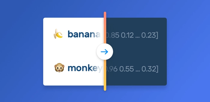
Ideally, we want vector representations where similar words end up with similar vectors. For that, we’ll create dense vectors (where the values are not only 0s and 1s but any decimal between them). So, instead of having a vector for Monkey equal to [1, 0, 0] as before, we’ll have something like [0.96, 0.55 … 0.32] and it’ll have a dimension (the amount of numbers) that we choose.
Even better, we’d want more similar representations when the words share some properties such as if they’re both plural or singular, verbs or adjectives or if they both reference to a male. All of those characteristics can be encoded in the vectors. And that’s exactly what Word2Vec showed in 2013 and changed the text vectorization field.
Goals and evaluation metrics
So, we want the vectors to better represent the words, but what does that mean? And how do we know if it's doing that well?
There are basically two kind of ways to know how they are performing: explicit methods and implicit methods.
Explicit methods
- Human evaluation: The first method is just as simple as taking some words, measuring the distance between the vectors generated for each of them and asking someone what they think about it. If they are a linguist, all the better. However, this is not scalable, time consuming, and requires thousands, even millions of words every time you get new vectors.
- Syntactic analogies: As dumb as it can sound, remember that word vectors are vectors, so we can add and subtract them. Thus, we generate tests of the form “eat is to eating as run is to ___”, then we make the operation eating - eat + run and find the most similar vector to that result. As you may have guessed, it should be the one correspondent to running.
- Semantic analogies: These are almost the same as the syntactic ones, but in this case the analogies will look more like “monkey is to animal as banana is to ___”, and we expect fruit as the result. We can even make more complex analogies as monkey + food = banana.
Take a moment to think about that: if we can make our vectors succeed in that kind of tests, it means that they are capturing the form and meaning of the words. It’s almost as if they are understanding the words.
Implicit methods
But hey, as exciting and wonderful as it sounds, it seems unlikely that having word-vectors is the real solution for a real-world problem. They are just a tool to make all the cool and really useful things we can do with NLP.
So, implicit methods are as simple as using the word vectors in some NLP task and measure their impact. If they make your algorithm work better, they’re good!
If you are working, for example, in a sentiment analysis classifier, an implicit evaluation method would be to train the same dataset but change the one-hot encoding, use word embedding vectors instead, and measure the improvement in your accuracy. If your algorithm gets better results then those vectors are good for your problem. Furthermore, you could train or get a new set of vectors and train again with those, and compare which one gets better results, meaning they are even better for that case.
As you can imagine, this can be very very expensive because it involves a lot of experimentation and testing what works better. Thus, it does not only means creating various sets of vectors but also training your algorithm with each of them (probably many times, as you’d want to adjust the hyperparameters to be fair in the comparison). That means a lot of time and computational resources.
How are word vectors created?
Well, we know what word vectors are, we know why we want them and we know how they should be. But, how do we get them?
As we already said, the main idea is to train over a lot of text and capture the interchangeability of the words and how often they tend to be used together. Are you wondering how much is “a lot of text”? Well, that’s usually in the order of the billions of words.
There are three big families of word vectors and we’re going to briefly describe each of them.
Statistical methods
Statistical methods work by creating a co-occurrence matrix. That is: they set a window size N (this is usually between 2 and 10). Then, they go through all the text and count how many times each pair of two words are together, meaning they are separated by as many as N words.
Say for the sake of example that our entire training set is just two texts: “I love monkeys” and “Apes and monkeys love bananas” and we set our window size N=2. Our matrix would be:
| Co-occurrence matrix | I | love | monkeys | and | apes | bananas |
|---|---|---|---|---|---|---|
| I | 0 | 1 | 1 | 0 | 0 | 0 |
| love | 1 | 0 | 2 | 1 | 0 | 1 |
| monkeys | 1 | 2 | 0 | 1 | 1 | 1 |
| and | 0 | 1 | 1 | 0 | 1 | 0 |
| apes | 0 | 0 | 1 | 1 | 0 | 0 |
| bananas | 0 | 1 | 1 | 0 | 0 | 0 |
Then, you apply some method for matrix dimensionality reduction such as Singular-Value Decomposition and voilà, each row of your matrix is a word vector. In case you are wondering what is a dimensionality reduction: when there’s redundant data in a matrix you can generate a smaller one with almost the same information. There are a lot of algorithms and ways to do it, usually they’re all related to finding the eigenvectors.
However nothing is easy, as Zaza Pachulia would say, and we still have some problems to solve:
The co-occurrence number alone is not a good number to measure the co-occurrence probability of two words because it does not take into account how many times each of them occur.
Imagine the words “the” and “monkey”, their co-occurrence in the texts will be very big, but that’s mainly because the occurrence of “the” is huge (we use it a lot). To solve this problem, usually we invoke the PMI (Pointwise Mutual Information), and we estimate the probabilities from the co-occurrences.
Think it this way: p(“the”) is so big, that the denominator will be much bigger than the numerator, so the number will be close to log(0) = a negative number. On the other hand, p(“monkey”) and p(“banana”) will not be even closer to p(“the”) because we don’t use them as much, so they won’t be as as many occurrences in the texts. In addition, we'll find a lot of texts where they appear together. In other words: the probability of co-occurrence will be high making the PMI for "monkey" and "banana" also a high number. Finally, when two words co-occur very little, the result will be the log of near 0: a very low negative number.![]()
This PMI method leads to many log(0) (i.e. −∞) entries (every time two words do not co-occur). Also the matrix is dense, there are not many zeros in it, that’s not good computationally, and remember we’re talking about a HUGE matrix. What is sometimes done is to use the Positive PMI, just max(PMI, 0) instead, to solve both problems. The intuition behind PPMI is that words with negative PMI have “less than expected” co-occurrences, which is not very valuable information and can be just caused by having insufficient amount of text.
The computation time in order to count all this is very expensive, especially if it’s done naively. Fortunately, there are ways to do this requiring just a single pass through the entire corpus to collect the statistics.


Predictive methods
Predictive methods work by training a Machine Learning algorithm to make predictions based on the words and their contexts. Then, they use some of the weights that the algorithm learns to represent each word. They are sometimes called neural methods, because they usually use neural networks.
Actually, the use of neural networks to create word embeddings is not new: the idea was present in this 1986 paper. However, as in every field related to deep learning and neural networks, computational power and new techniques have made them much better in the last years.
The first approaches were usually made using neural networks and training them to predict the next word in a text given the previous N words. The important thing here is that the neural network is trained to get better in that task, but you don’t really care about that result: all you generally want are the weights of the matrix that represent the words.
One big example of this kind of approach is a paper published by Bengio et. al. in 2003, a very important paper in the field, where they use a neural network with one hidden-layer to do it.
And then, the breakthrough, the work that put word embeddings into the cool status, the one you were probably waiting for: Word2vec.
Mikolov et al. focused on performance: they removed the hidden layers of the neural network in order to make them train much faster. That may sound as losing “learning power”, and it is actually, but the fact that you can train with a huge amount of data, even hundreds of billions of words not only makes up for it, but also has been proven to produce better results.
In addition, they presented two variants of the training and many optimizations that apply to both of them. Let’s take a closer look at each:
Continuous Bag of Words (CBOW)
The basic idea here is to set a sliding window of size N, in this case, let say N is 2. Then you take a huge amount of text and train a neural network to predict a word inputting the N words at each side.
Imagine that you have the text “The monkey is eating a banana”, you will try to predict the word is given that the two previous words are The and monkey and the next two are eating and a. Also, you’ll train to predict eating knowing the four surrounding words are monkey, is, a and banana. And go on with all the text.
And remember, the neural network is a very small one, let’s go over it step by step:


In CBOW we try to predict the word "eating" given the one-hot encoded vectors of it's context. In skip-gram we try to predict the context given the word "eating"
- It has an input layer that receives four one-hot encoded words which are of dimension V (the size of the vocabulary).
- It averages them, creating a single input vector.
- That input vector is multiplied by a weights matrix W (that has size VxD, being D nothing less than the dimension of the vectors that you want to create). That gives you as a result a D-dimensional vector.
- The vector is then multiplied by another matrix, this one of size DxV. The result will be a new V-dimensional vector.
- That V-dimensional vector is normalized to make all the entries a number between 0 and 1, and that all of them sum 1, using the softmax function, and that’s the output. It has in the i-th position the predicted probability of the i-th word in the vocabulary of being the one in the middle for the given context.
That’s it. Oh, are you wondering where are the word vectors there? Well, they are in that W weights-matrix. Remember we said it’s size is VxD so the row i is a D-dimensional vector representing the word i in the vocabulary.
In fact, think that if you had just one word used as context, your input vector would be a one-hot encoded representation of that word, and multiplying it by W would be just like selecting the corresponding word vector: everything makes sense, right?
Skipgram
Skipgram is just the same as CBOW, but with one big difference: instead of predicting the word in the middle given all the others, you train to predict all the others given the one in the middle.
Yes, knowing just one word it tries to predict four. I’ve been familiar with word2vec for a while now and this idea still blows my mind. It seems absurd, but, hey, it works! And it actually works a little better than CBOW.
Apart from the algorithms, word2vec proposed many optimizations to them, such as:
- Give more weight to the closer words in the window.
- Remove rare words (that only appear a few times) from the texts.
- Treating the common word pairs like “New York” as a single word.
- Negative sampling: it’s a technique to improve the training time. When you train with one word and it’s context, you usually update all of the weights in the neural network (remember there a lot of them!). With negative sampling you just update the weights that correspond to the actual word that should have been predicted and some other randomly chosen words (the suggest to select between 2 and 20 words), letting most of them as they were.If you want to understand more about negative sampling, I recommend you to read this nice blogpost about it. Negative sampling is so important that you’ll frequently see the algorithm referred as SGNS (Skip-Gram with Negative Sampling)
Combined methods
As usual, when two methods give good results, you can achieve even better results combining them. In this case that means training a machine learning model and getting the word vectors from the weights of it, but instead of using a sliding-window to get the contexts, train using the co-occurrence matrix.
The most important of this combined methods is GloVe. They created an algorithm that consists in a very simple machine learning algorithm (a weighted least squares regression) that trains to create vectors that satisfy that if you take the vector of two words i and j and multiply them, the result is similar to the logarithm of the ij entry in the co-occurrence matrix, i.e. the number of co-occurrences for those two words.
They also make some optimizations like adding some weighting to prevent rare co-occurrences to introduce noise and very common ones to skewing the objective too much.
They make explicit and implicit methods for testing (remember them?) getting really good results.
5 Myths you shouldn’t believe
I hope that by this time you know what word vectors are, how to know if some set of vectors are good, and to have at least an idea of how they are created.
But as usually happens when something gains cool status, there are some widespread ideas that I’d like to clarify that are not true:
1. Word2vec is the best word vector algorithm
This is not true in many senses. In the most simple sense: word2vec is not an algorithm, it is a group of related models, tests and code. They introduced actually two different algorithms in word2vec, as we explained before: Skip-gram and CBOW. Also, when it was first published, the results it got were definitely better than the state of the art. But it’s important to notice that they presented, besides the algorithms, many optimizations that were translated to statistical methods improving their results to a comparable (sometimes even better) level. This great paper explains which are this optimizations and how they were used to improve the statistical methods.
2. Word vectors are created by deep learning
This is just plainly not true. As you know if you’ve thoughtfully read this post, some vectors are created with statistical methods, and there isn’t even a neural network involved there, let alone a deep neural network.
And, actually, one of the most important changes to predictive methods introduced in word2vec was to remove the hidden layers of the neural networks, so it would be really wrong to call that neural network “deep”.
3. Word vectors are used only with deep learning
Word vectors are great to use as the input of deep learning models, but that’s not exclusive. They are also great to feed SVM, MNB or almost any other machine learning model that you can think of.
4. Statistical and predictive methods have nothing to do with each other
They were created separately as different approaches to the problem of creating vectors, but they can be combined, as we’ve seen with GloVe, and some techniques can be applied to both of them.
In fact it has been proved that Skip-Gram with Negative Sampling implicitly factorizes a PMI matrix shifted by a global constant. A very important result because it relates the two worlds of statistical and predictive methods.
5. There’s a perfect set of word vectors that can be used in every NLP project
You’ve got to the last part of this post, so I’m assuming you know this already: word vectors are context dependent, they are created learning from text.
So, if you trained your vectors with English news, the football vector will be similar to, say, goal, forward, midfielder, goalkeeper and Messi. On the other hand, if you trained your vectors with American news, the football vector will be similar to touch-down, quarterback, fullback and Brady.
This is a characteristic that you need to take into account, especially when working in specific domain problems.
Having said that, one of the biggest impact of word vectors is that they are really really good when used in transfer learning: the field of using knowledge learned solving a problem to solve another one. Moreover, it’s very unusual to train your vectors from scratch when starting a project, in most cases you start with a set of already-created vectors and train them with your specific texts.
Conclusion
Word embeddings are not new, but the progress made in the field in the last years have pushed them into the state of the art of NLP. Not only the computational power has allowed to train them much faster and process huge amounts of text, but also many new algorithms and optimizations have been created.
In this post, we’ve presented the basics of how do most of those algorithms work, but there are many other tricks and tweaks to discover. Also, there are new trends like the subword level embeddings implemented in the FastText library (I tell you, we love FastText here in MonkeyLearn, it’s so fast!), other libraries like StarSpace, and many more interesting things.
Word embeddings are fun to play with, not so difficult to understand, and very useful in most NLP tasks, so I hope you’d enjoyed learning about them!


Gabriel Mordecki
December 7th, 2017
Posts you might like...


Text Analysis with Machine Learning
Turn tweets, emails, documents, webpages and more into actionable data. Automate business processes and save hours of manual data processing.
Try MonkeyLearn


